Wide field fluorescence lifetime imaging microscopy

R. Murray, from the National University of Ireland used the 4 Picos intensified CCD camera with a shortest gating time of 200ps to construct a wide field fluorescence lifetime imaging microscope (wide field FLIM) system with sub-nanosecond resolution.

Schematic of the wide field FLIM setup. The pulsed excitation light source is directed toward the reflected light port of the microscope. Upon entering the microscope, the excitation passes through a clean up filter and illuminates the sample stage via the microscope objective. The fluorescence emission is collected by the objective and directed toward the 4 Picos ICCD camera. The data is passed to a PC for data analysis and determination of the fluorescence lifetime map.

Lifetime fluorescence measurement with sub-nanosecond resolution

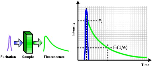
Fluorescence is the phenomenon in which a molecule absorbs light, and subsequently emits light of a different, typically longer, wavelength. The fluorescence lifetime of a molecule is the average time the molecule spends in the excited state before returning to the ground state by emission of a fluorescence photon. If dealing with a single fluorescent species in a homogenous environment, then the intensity can be described by a mono-exponential decay function. However, it is common to encounter mixtures of fluorescent species that display multi-exponential decay functions within a fluorescent system. These fluorescent systems may emit fluorescence at different wavelengths and also have different lifetimes. Therefore, these measurements can be described using a multi-exponential decay model.

Experimental setup of the wide field FLIM

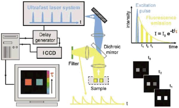
The basic consideration of the experimental setup is the illumination of the sample using a 405nm pulsed laser diode and collect the shifted fluorescence signal with the ICCD camera. Therefore, a beam-splitter is used within the microscope to separate the primary laser pulse from the fluorescence signal. This beam-splitter reflects the excitation wavelength of 405nm and transmits the fluorescence signal of the sample which is shifted longer wavelengths. The experimental wide field FLIM setup needs additionally a trigger synchronisation of the pulsed laser diode and the intensified CCD camera.

Simple representation of time domain lifetime measurements. The excitation pulse is incident on the sample causing fluorescence to be emitted. The emitted fluorescence decays exponentially. And is sampled prior to lifetime calculations

Measuring lifetime fluorescence using a ICCD camera

There are two broad classes of measurement technique that can be employed in fluorescence measurements, namely steady-state, and time-resolved measurements. In contrast to the steady-state measurement the excitation source of time-resolved measurements is either pulsed or modulated which enables the measurement of fluorescence emission and kinetics. Time domain fluorescence measurement methods are generally more easily understood because they generate a true representation of the fluorescence decay curve (see the figure above). Typically time domain systems consist of a pulsed light source providing excitation coupled with a fast response detector.

Time Correlated Single Photon Counting vs. wide field FLIM

The methods for time domain lifetime measurements can be generally classified into two groups, namely single point measurements and wide field measurements. A common single point measurement method is Time Correlated Single Photon Counting (TCSPC) which normally uses either a PMT or SAPDas the detection module. Wide field lifetime measurements systems use intensified CCD cameras as the detection module. In both measurement methods the sample is excited by the pulsed excitation source. The detectors then build up the fluorescence decay curve by sampling portions of the decay curve and then reconstructing it using either electronics or software. Once the decay curve has been reconstructed the lifetime can be calculated by fitting an appropriate fitting to the collected data. The difference of the two methods is the way they create a 2D fluorescence map. The TCSPC is scanning the excitation source across the sample and is determine the corresponding fluorescence lifetime values in a consecutive series. The wide field FLIM excites the complete sample at once and the lifetime fluorescence can be individually calculated from each pixel position of the detector.

Wide field FLIM signal collection as time delayed image sequence and analysis of 2D fluorescent lifetime map. (A) Shows the data capture sequence where the fluorescence decreases with increasing delay time (t1– t4). (B) During the data analysis the signal decay curve for each individual pixel need to be calculated. For reconstruction of the decay curve, a fitting model is assigned to the data and the fluorescent lifetime is calculated for each individual pixel. As a result the fluorescence lifetime is plotted in a 2D image which is called the FLIM map.

Wide field FLIM measurements for sub-nanosecond lifetime validation

Lifetime validation measurements were made using standards samples which has a known lifetime. Two samples were chosen (HPTS and Coumarin30) because they have both very stable lifetimes in combination with relatively broad emission spectra. The wide field FLIM images generated for both standards are shown in the figure below.

Wide Field FLIM images of HPTS, on the left, and Coumarin 30, on the right. The accepted lifetime values for HPTS and Coumarin 30 are 5.4ns and 2.4ns respectively. The wide field FLIM system determined the lifetimes of HPTS with 5.5ns ±0.1ns and Coumarin 30 with 2.1ns ±0.1ns.

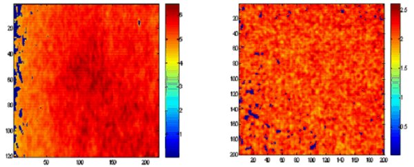
It was shown that over the investigated region the lifetime of the samples was determined with 5.4ns ±0.1 ns and 2.1ns ±0.1ns for HPTS and Coumarin 30, respectively. Therefore, the wide field FLIM measurements agrees with the reported lifetime values for HPTS which is 5.4ns. There is a close agreement between the wide field FLIM lifetime value and the reported value for Coumarin 30 of 2.4ns. This indicates that the fluorescence lifetime measurement with sub-nanosecond resolution are possible with the 4 Picos intensified CCD camera.

Wide field FLIM measurements and conclusion

R. Murray used the wide field FLIM setup to analyze hydrocarbon bearing fluid inclusion (HCFI) of crude oil. Since this method does not use the measured intensity directly, it represents a very robust measurement methodology. However, the results showed that the reported lifetime measurements by the wide field FLIM system exhibit unexpected uncertainties. The lifetime results obtained using the wide field FLIM may be improved by increasing the number of time gates and by further development the fitting algorithm used in MATLAB to account for multi-exponential decay fitting. As such, caution must be exercised in using the wide field FLIM reported lifetimes. Nevertheless, the wide field fluorescence lifetime measurements are very useful for fast 2D lifetime contrast imaging and determining the homogeneity of the sample.

---

Title: The Development of a Wide-Field Fluorescence Lifetime Imaging Microscope
(WF-FLIM) System for Petro-Geological Analysis
Author: Richard Murray (Ph.D Thesis)
Institute: National University of Ireland, Galway, Ireland